
- Introduction
- Graphing Solutions of Cubic Equations
- Average Rate of Change
- Empirical Graphs
- Reduction of Non-linear Laws to Linear Form.
- Equation of a Circle
- Past KCSE Questions on the Topic.

Introduction
- These are ways or methods of solving mathematical functions using graphs.
Graphing Solutions of Cubic Equations
- A cubic equation has the form
ax3 + bx2 + cx + d = 0
where a, b , c and d are constants - It must have the term in x3 or it would not be cubic (and so a ≠ 0), but any or all of b, c and d can be zero. For instance,
x3 − 6x2 + 11x −6 = 0, 4x3 + 57 = 0, x3 + 9x = 0
are all cubic equations. - The graphs of cubic equations always take the following shapes.
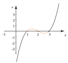
y =x3 −6x2 + 11 x −6 = 0. - Notice that it starts low down on the left, because as x gets large and negative so does x3 and it finishes higher to the right because as x gets large and positive so does x3. The curve crosses the x-axis three times, once where x = 1 , once where x = 2 and once where x = 3. This gives us our three separate solutions.
Example
- Fill in the table below for the function y = −6 + x + 4x2 + x3 for −4 ≤ x ≤2
x −4 −3 −2 −1 0 1 2 −6 −6 −6 −6 −6 −6 −6 −6 x −4 −3 −2 −1 0 1 2 4x2 16 4 x3 y - Using the grid provided draw the graph for y = −6 + x + 4x2 + x3 for −4≤x ≤2
- Use the graph to solve the equations:-
- −6 + x + 4x2 + x3 = 0
- x3 + 4x2 + x – 4 = 0
- −2 + 4x2 + x3 = 0
Solution
The table shows corresponding values of x and y for y = −6 + x + 4x2 + x3
| X | −4 | −3 | −2 | −1 | 0 | 1 | 2 |
| −6 | −6 | −6 | −6 | −6 | −6 | −6 | −6 |
| X | −4 | −3 | −2 | −1 | 0 | 1 | 2 |
| 4x2 | 64 | 36 | 1 6 | 4 | 0 | 4 | 1 6 |
| X3 | −64 | −27 | −8 | −1 | 0 | 1 | 8 |
| Y=−6+x+4x2 +x3 | −10 | 0 | 0 | −4 | −6 | 0 | 20 |
From the graph the solutions for x are x = −3 , x = −2, x = 1
To solve equation y = −6 + x + 4x2 + x3 we draw a straight line from the diffrence of the two equations and then we read the coordinates at the point of the intersetion of the curve and the straight line
y = x3 + 4x2 + x − 6
0 = x3 + 4x2 + x − 4
y = –2 solutions 0.8, −1.5 and −3.2
| x | 1 | 0 | −2 |
| y | −3 | −4 | −8 |
y = x3 + 4x2 + x – 6
0 = x3 + 4x2 + 0 – 2
y = x – 4

Average Rate of Change
Defining the Average Rate of Change
- The notion of average rate of change can be used to describe the change in any variable with respect to another. If you have a graph that represents a plot of data points of the form (x, y), then the average rate of change between any two points is the change in the y value divided by the change in the x value.
Note; - The rate of change of a straight ( the slop)line is the same between all points along the line
- The rate of change of a quadratic function is not constant (does not remain the same)
- The average rate of change of y with respect to x = change in y
change in x
Example
The graph below shows the rate of growth of a plant,from the graph, the change in height between day 1 and day 3 is given by 7.5 cm – 3.8 cm = 3.7 cm.
Average rate of change is 3.7 cm/2 days = 1.85 cm/day
The average rate of change for the next two days is 1.3 cm/2 days = 0.65cm/day
Note;
- The rate of growth in the first 2 days was 1.85 cm/day while that in the next two days is only 0.65 cm/day. These rates of change are represented by the gradients of the lines PQ and QR respectively.

- The gradient of the straight line is 20 ,which is constant. The gradient represents the rate of distance with time (speed) which is 20 m/s.

Rate of Change at an Instant
We have seen that to find the rate of change at an instant (particular point), we:
- Draw a tangent to the curve at that point
- Determine the gradient of the tangent
The gradient of the tangent to the curve at the point is the rate of change at that point.
Empirical Graphs
An Empirical graph is a graph that you can use to evaluate the fit of a distribution to your data by drawing the line of best fit. This is because raw data usually have some errors.
Example
The table below shows how length l cm of a metal rod varies with increase in temperature T (0C).
| Temperature oC | 0 | 1 | 2 | 3 | 5 | 6 | 7 | 8 |
| Length cm | 4.0 | 4.3 | 4.7 | 4.9 | 5.0 | 5.9 | 6.0 | 6.4 |
Solution

NOTE;
- There is a linear relation between length and temperature.
- We therefore draw a line of best fit that passes through as many points as possible.
- The remaining points should be distributed evenly below and above the line

The line cuts the y – axis at (0, 4) and passes through the point (5, 5.5).Therefore, the gradient of the line is 1.5/5 = 0.3.The equation of the line is l =0.3T + 4.
Reduction of Non-linear Laws to Linear Form.
- When we plot the graph of xy=k, we get a curve.But when we plot y against 1/x , w get a straight line whose gradient is k.The same approach is used to obtain linear relations from non-linear relations of the form y= kxn.
Example
The table below shows the relationship between A and r
| r | 1 | 2 | 3 | 4 | 5 |
| A | 3.1 | 1 2.6 | 28.3 | 50.3 | 78.5 |
It is suspected that the relation is of the form A=Kr2.By drawing a suitable graph,verify the law connecting A and r and determine the value of K.
Solution
If we plot A against r2,we should get a straight line.
| r | 1 | 2 | 3 | 4 | 5 |
| A | 3.1 | 12.6 | 28.3 | 50.3 | 78.5 |
| r2 | 1 | 4 | 9 | 16 | 25 |

Since the graph of A against r2 is a straight line, the law A =kr2 holds. The gradient of this line is 3.1 to one decimal place. This is the value of k.
Example
From 1960 onwards, the population P of Kisumu is believed to obey a law of the form P =kAt,Where k and A are constants and t is the time in years reckoned from 1960.The table below shows the population of the town since 1960.
| r | 1960 | 1965 | 1970 | 1975 | 1980 | 1985 | 1990 |
| P | 5000 | 6080 | 7400 | 9010 | 10960 | 13330 | 16200 |
By plotting a suitable graph, check whether the population growth obeys the given law. Use the graph to estimate the value of A.
Solution
The law to be tested is P=kAt. Taking logs of both sides we get log P =log(kAt). Log P = log K + t log A, which is in the form y = mx + c. Thus we plot log P against t.
(Note that log A is a constant).
The table below shows the corresponding values of t and log p.
| r | 1960 | 1965 | 1970 | 1975 | 1980 | 1985 | 1990 |
| Log P | 3.699 | 3.784 | 3.869 | 3.955 | 4.040 | 4.125 | 4.210 |
Since the graph is a straight line, the law P =kAt holds.
Log A is given by the gradient of the straight line.Therefore, log A = 0.017.
Hence, A = 1.04
Log k is the vertical intercept.
Hence log k =3.69
Therefore k = 4898
Thus, the relationship is P = 4898(1.04)t
Note;
- Laws of the form y=kAx can be written in the linear form as: log y = log k + x log A (by taking logs of both sides)
- When log y is plotted against x , a straight line is obtained.Its gradient is log A and the intercept is log k.
- The law of the form y =kXn,where k and n are constants can be written in linear form as; Log y = log k + n log x.
- We therefore plot log y is plotted against log x.
- The gradient of the line gives n while the vertical intercept is log k
Summary
For the law y = d + cx2 to be verified it is necessary to plot a graph of the variables in a modified form as follows
y = d +cx2 is compared with y = mx + c that is y =cx2 + d
- Y is plotted on the y axis
- x2 is plotted on the x axis
- The gradient is c
- The vertical axis intercept is d
For the law y – a = b x to be verified it is necessary to plot a graph of the variables in amodified form as follows
y – a = b√x , i.e. y = b√x + a which is compared with y = mx + c
- y should be plotted on the y axis
- x should be plotted on the x axis
- The gradient is b
- The vertical axis intercept is a
For the law y – e = f/x to be verified it is necessary to plot a graph of the variables in a modified form as follows.
The law y – e = f/x is f (1/x) + e compared with y = mx + c.
- y should be plotted on the vertical axis
- 1/x should be plotted on the horizontal axis
- The gradient is f
- The vertical axis intercept is e
For the law y – cx = bx2 to be verified it is necessary to plot a graph of the variables in a modified form as follows.
The law y – cx = bx2 is y/x= bx + c compared with y = mx + c,
- y/x should be plotted on y axis
- X should be plotted on x axis
- The gradient is b
- The vertical axis intercept is c
For the law y = a/x + bx to be verified it is necessary to plot a graph of the variables in a modified form as follows.
The law y = a + b compared with y = mx + c
- y/x should be plotted on the vertical axis
- 1/x2 should be plotted on the horizontal axis
- The gradient is a
- The vertical intercept is b
Equation of a Circle
- A circle is a set of all points that are of the same distance r from a fixed point. The figure below is a circle centre (0,0) and radius 3 units

- P (x ,y ) is a point on the circle. Triangle PON is right – angled at N.
By Pythagoras’ theorem;
ON2 + PN2 = OP2
But ON = x, PN = y and OP = 3 .Therefore, x2 + y2 = 32
Note; - The general equation of a circle centre (0, 0) and radius r is x2 + y2 = r2
Example
Find the equation of a circle centre (0, 0) passing through (3, 4)
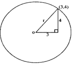
Solution
Let the radius of the circle be r
From Pythagoras theorem;
r = √(32 x 42)
r = 5
Example
Consider a circle centre (5 , 4 ) and radius 3 units.

Solution
In the figure below triangle CNP is right angled at N.By pythagoras theorem;
CN2 + NP2 = CP2
But CN= (x – 5), NP = (y – 4) and CP =3 units.
Therefore,(x – 5)2 + (y – 4 )2 = 32 this is the equation of a circle.
Note;
The equation of a circle centre ( a,b) and radius r units is given by;
(x–a)2 + (y–b)2 = (r)2
Example
Find the equation of a circle centre (–2 ,3) and radius 4 units
Solution
General equation of the circle is (x–a)2 + (y–b)2 = r2 .Therefore a = –2, b =3 and r = 4
(x–(–2))2 + (y–(3))2 = 42
(x+2)2 + (y–3)2 = 16
Example
Line AB is the diameter of a circle such that the co-ordinates of A and B are (–1, 1 ) and(5, 1 ) respectively.
- Determine the centre and the radius of the circle
- Hence, find the equation of the circle
Solution
- (–1+5, 1+21) = (2,1)
2 2
Radius =√[(5–2)2 + (1–1)2]
=√32 = 3 - Equation of the circle is ;
(x–2)2 + (y–1)2 = 32
(x–2)2 + (y–1)2 = 9
Example
The equation of a circle is given by x2 – 6x + y2 + 4y – 3 = 0.Determine the centre and radius of the circle.
Solution
x2 – 6x +y2 + 4y = 3
Completing the square on the left hand side;
x2 – 6x + 9+y2 + 4y + 4 = 3 + 9 + 4
(x – 3)2 + (y + 2)2 = 4 – 3 = 0
Therefore centre of the circle is (3,–2) and radius is 4 units. Note that the sign changes to opposite positive sign becomes negative while negative sign changes to positive.
Example
Write the equation of the circle that has A(1, – 6) and B(5, 2) as endpoints of a diameter.
Solution
Method 1:
Determine the center using the Midpoint Formula:
C(1+5 , –6+2)→C(3, –2)
2 2
Determine the radius using the distance formula (center and end of diameter):
r = (3−1)2 + (−2+6)2 = √(4 + 16) = 20 = 2√5
Equation of circle is: (−3)2 + (y+2)2 = 20
Method 2:
Determine center using Midpoint Formula (as before): C(3,−2).
Thus, the circle equation will have the form (x−3)2 + (y+2)2 = r2
Find r2 by plugging the coordinates of a point on the circle in for x and y.
Let’s use B(5, 2):r2 = (5−3)2 + (2+2)2 = 22 + 42 = 4 + 16 = 20
Again, we get this equation for the circle: (x−3)2 + (y+2)2 = 20
Past KCSE Questions on the Topic.
- The table shows the height metres of an object thrown vertically upwards varies with the time t seconds
The relationship between s and t is represented by the equations s = at2 + bt + 10 where b are constants.T 0 1 2 3 4 5 6 7 8 9 10 S 45.1 49.9 −80 -
- Using the information in the table, determine the values of a and b
- Complete the table
-
- Draw a graph to represent the relationship between s and t
- Using the graph determine the velocity of the object when t = 5 seconds
-
- Data collected form an experiment involving two variables X and Y was recorded as shown in the table below
The variables are known to satisfy a relation of the form y = ax3 + b where a and b are constantsx 1.1 1.2 1.3 1.4 1.5 1.6 y −0.3 0.5 1 .4 2.5 3.8 5.2 - For each value of x in the table above, write down the value of x3
- By drawing a suitable straight line graph, estimate the values of a and b
- Write down the relationship connecting y and x
- Two quantities P and r are connected by the equation p = krn. The table of values of P and r is given below.
P 1.2 1.5 2.0 2.5 3.5 4.5 R 1.58 2.25 3.39 4.74 7.86 11 .5 - State a liner equation connecting P and r.
- Using the scale 2 cm to represent 0.1 units on both axes, draw a suitable line graph on the grid provided. Hence estimate the values of K and n.
- The points which coordinates (5,5) and (−3,−1 ) are the ends of a diameter of a circle centre A
Determine:- The coordinates of A
- The equation of the circle, expressing it in form x2 + y2 + ax + by + c = 0 where a, b, and c are constants each computer sold
- The figure below is a sketch of the graph of the quadratic function y = k(x+1 ) (x−2)
Find the value of k - The table below shows the values of the length X (in metres ) of a pendulum and the corresponding values of the period T (in seconds) of its oscillations obtained in an experiment.
X (metres) 0.4 1 .0 1 .2 1 .4 1 .6 T (seconds) 1 .25 2.01 2.1 9 2.37 2.53 - Construct a table of values of log X and corresponding values of log T, correcting each value to 2 decimal places
- Given that the relation between the values of log X and log T approximate to a linear law of the form m log X + log a where a and b are constants
- Use the axes on the grid provided to draw the line of best fit for the graph of log T against log X.
- Use the graph to estimate the values of a and b
- Find, to decimal places the length of the pendulum whose period is 1 second.
- Data collection from an experiment involving two variables x and y was recorded as shown in the table below
The variables are known to satisfy a relation of the form y = ax3 + b where a and b are constantsX 1.1 1.2 1.3 1.4 1.5 1.6 Y −0.3 0.5 1.4 2.5 3.8 5.2 - For each value of x in the table above. Write down the value of x3
-
- By drawing s suitable straight line graph, estimate the values of a and b
- Write down the relationship connecting y and x
- Two variables x and y, are linked by the relation y = axn. The figure below shows part of the straight line graph obtained when log y is plotted against log x.
Calculate the value of a and n - The luminous intensity I of a lamp was measured for various values of voltage v across it. The results were as shown below
It is believed that V and l are related by an equation of the form l = aVnwhere a and n are constant.V(volts) 30 36 40 44 48 50 54 L (Lux ) 708 1248 1726 2320 3038 3848 4380 - Draw a suitable linear graph and determine the values of a and n
- From the graph find
- The value of I when V = 52
- The value of V when I = 2800
- In a certain relation, the value of A and B observe a relation B= CA + KA2 where C and K are constants. Below is a table of values of A and B
A 1 2 3 4 5 6 B 3.2 6.75 10.8 15.1 20 25.2 - By drawing a suitable straight line graphs, determine the values of C and K.
- Hence write down the relationship between A and B
- Determine the value of B when A = 7
- The variables P and Q are connected by the equation P = abq where a and b are constants. The value of p and q are given below
P 6.56 1 7.7 47.8 1 29 349 941 2540 6860 Q 0 1 2 3 4 5 6 7 - State the equation in terms of p and q which gives a straight line graph
- By drawing a straight line graph, estimate the value of constants a and b and give your answer correct to 1 decimal place
Download Graphical Methods - Mathematics Form 3 Notes.
Tap Here to Download for 50/-
Get on WhatsApp for 50/-
Why download?
- ✔ To read offline at any time.
- ✔ To Print at your convenience
- ✔ Share Easily with Friends / Students